
Microsoft Excel can be very intimidating especially when you’re not an expert, like me. I was asked to write a blog on a topic I was not familiar with. I chose to challenge myself and learn more about Excel and the creation of PivotTables.
What is a PivotTable? A PivotTable is a tool that helps you calculate, summarize and analyze large amounts of data. It helps you make sense of it, all without copying and pasting or typing any formulas. Sounds interesting, but let’s see how easy it is.
Note: Microsoft has added PivotCharts to accentuate your data.
Let’s LEARN
First, open the document with the data you want displayed in a PivotTable. Make sure the data is in good shape. Name all your columns and be sure there is no duplicate information, or blank cells.
One thing to keep in mind when working with PivotTables, each column represents a “Field” in Excel. It’s a traditional term used when working with data and database applications.
Secondly, we need to make sure that your data is formatted as a table. To do that, select your Data, then click on the Home tab and select Format as Table. Here you will be given format and color options to select from. I’ve selected the Green Table Style Light 14.
 After you have made your Format Table selection, a dialog box will appear asking what data you want for your table. This is typically filled out by Excel, but you need to check off whether your table has headers or not. After you click “My table has headers,” click OK.
Note: Any other rows of data added to your spreadsheet after you have selected Table Format will automatically format to match the table you just created.
Creating a PivotTable
First, select the cells you want to create a PivotTable from and click Insert > PivotChart. 
A dialog box will appear asking for the Table/Range which is automatically filled out. Next, click on New Worksheet and then click OK.
Note: If you want the PivotTable on the existing spreadsheet you will need to specify location.
A New Worksheet will appear as a blank template.
Now we need to decipher what content we want displayed in our PivotTable.
Next, we will select the content we want our PivotTable/Chart to report. On the right-hand side of the screen you will see your PivotTable Fields Pane. Here you will select what data you want to display.

First, ask yourself the following questions:
- What do I want to be arranged in Axis (Categories/Rows)?
- What do I want to be displayed in the Legend (Series/Columns)?
- What do I want to be displayed in Values?
- What Filters, if any, do I want to apply?
Let’s say I want to know how much Sales and Marketing spent in the 2nd quarter. In order to display the results you will need to click and drag fields to one of the boxes below in the PivotChart Field Pane. In the sample below, I placed Department in the Axis box/rows, Sum of Amount in the Values box, the Item in the Legend/columns, and since I want to filter by Quarter, I placed Quarter in the Filter box.
When you place each field in a box, your data will automatically place a value in the table and the chart. However, you will need to resort back to the PivotTable to select what you want to be filtered. (see Screenshot 2)
I selected the 2nd Quarter information to be displayed.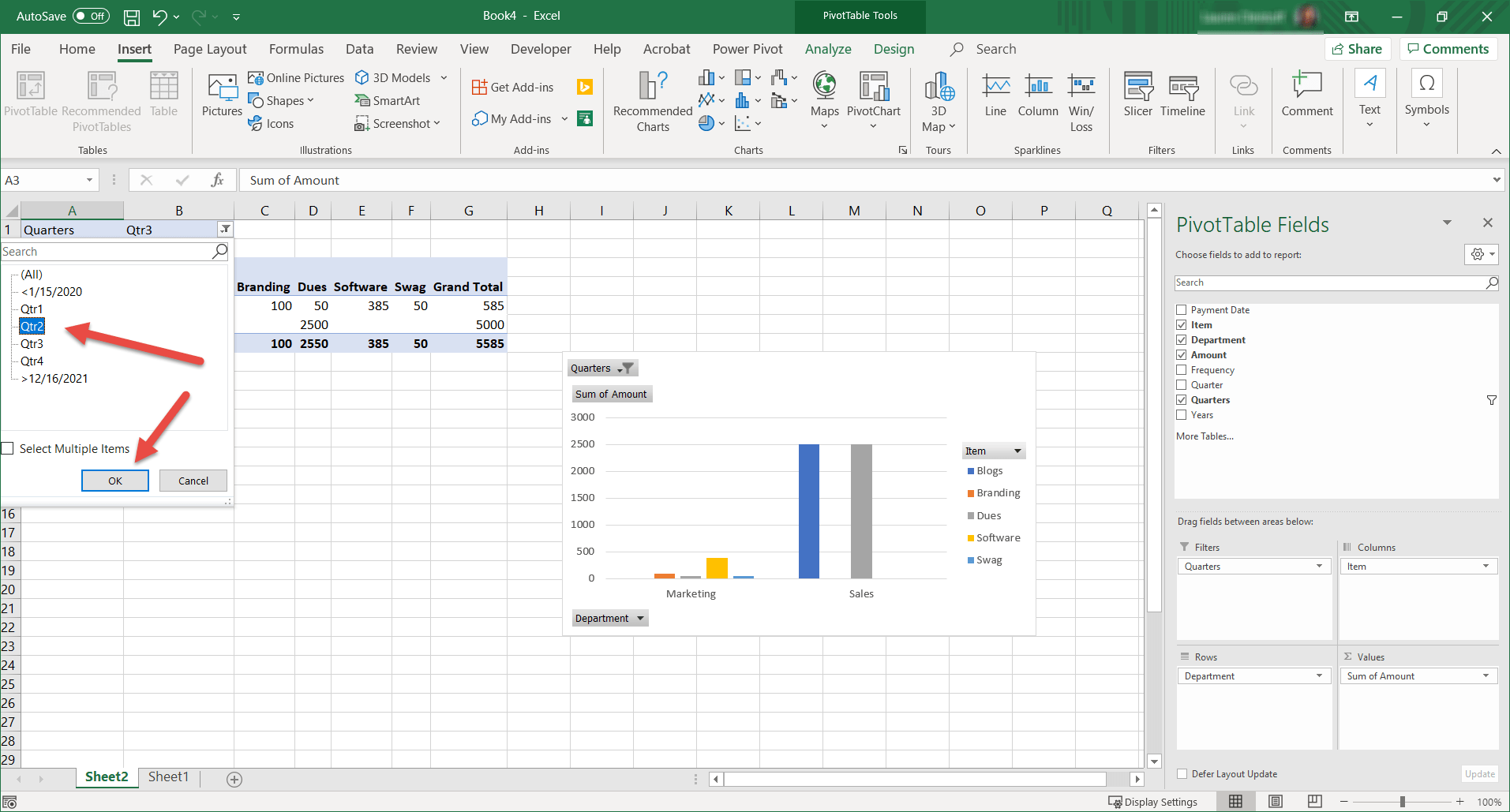
After you click OK, both the PivotTable and PivotChart will calculate the values and display that information.
If you later decide that you don’t want to see a certain field displayed on the Table or Chart, you can simply remove that field by clicking on the down arrow on the field you want to remove and select Remove Field. You can also select other attributes for that specific Field as you see fit.
I removed Item from the Legend/columns section. Here are my results:
If you make a mistake or are not sure if the information displayed is what you want to see, you can always create additional PivotTables and Charts by simply going back through the steps above and create a New Worksheet and play around with the different fields by placing them in the different areas.
That wraps up how to create PivotTables and PivotCharts, I hope you found this how-to helpful. For more Tips & Tricks check be sure to subscribe to our blog.